A few figures from my work on sharp-interface cut-cell methods: how the discretisation
behaves on adaptive meshes, how interface conditions are imposed, and what the resulting
accuracy looks like.
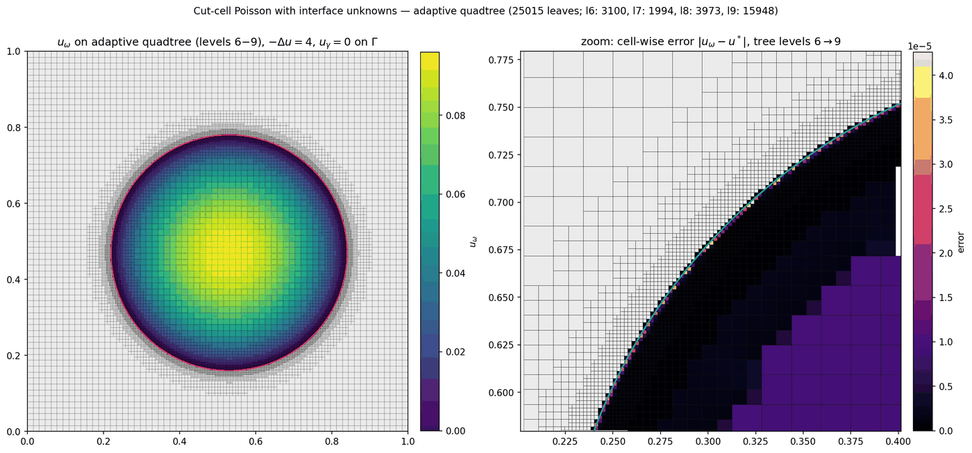
Cut-cell Poisson with interface unknowns, on an adaptive quadtree.
The solution of −Δu = 4 with a homogeneous
condition on the immersed boundary Γ, over a mesh spanning levels 6 to 9
(25 015 leaves). Refinement concentrates where it is needed, along the interface.
The zoom shows the cell-wise error against the exact solution: it stays below
4 × 10⁻⁵, and the cut cells are no worse than the
bulk, which is the point of carrying unknowns on the interface itself.
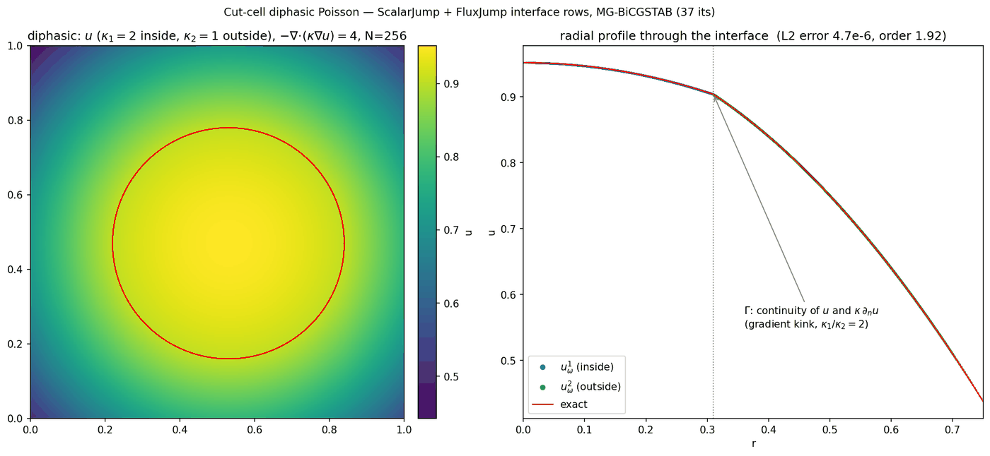
Two-phase Poisson across a curved interface.
Here both phases are solved at once, with a conductivity ratio
κ1/κ2 = 2, coupled by
scalar and flux jump conditions written directly on the interface rows of the system.
The radial profile makes the coupling visible: the solution is continuous through
Γ while its gradient kinks, exactly as continuity of
κ ∂nu requires. The measured
L2 error is 4.7 × 10⁻⁶, at observed order 1.92.
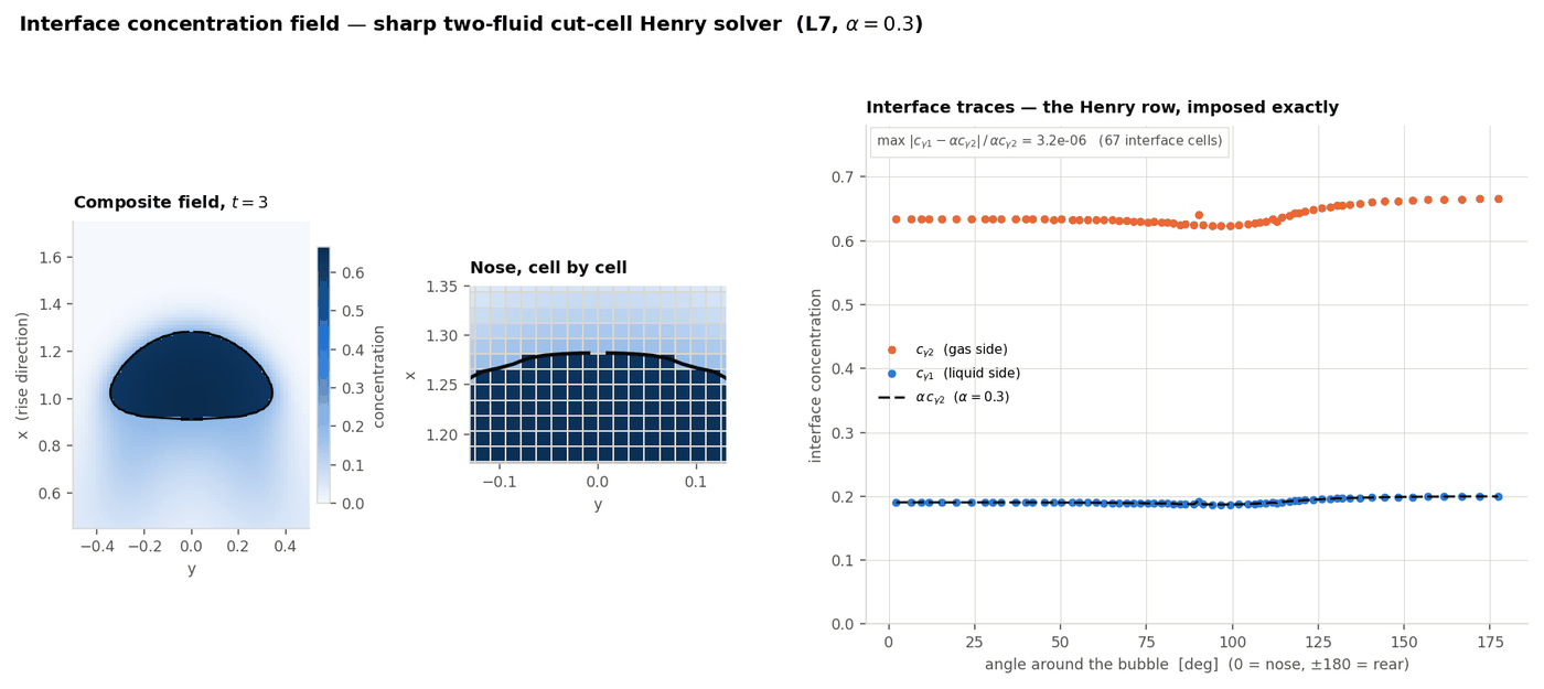
Interface concentration around a rising bubble.
A sharp two-fluid solver for mass transfer, where the concentration is discontinuous
at the interface: the liquid and gas traces are related by Henry's law,
cγ1 = α cγ2.
Plotting both traces cell by cell around the bubble shows the condition is imposed to
3.2 × 10⁻⁶ relative, over all 67 interface cells,
rather than smeared over a transition band.
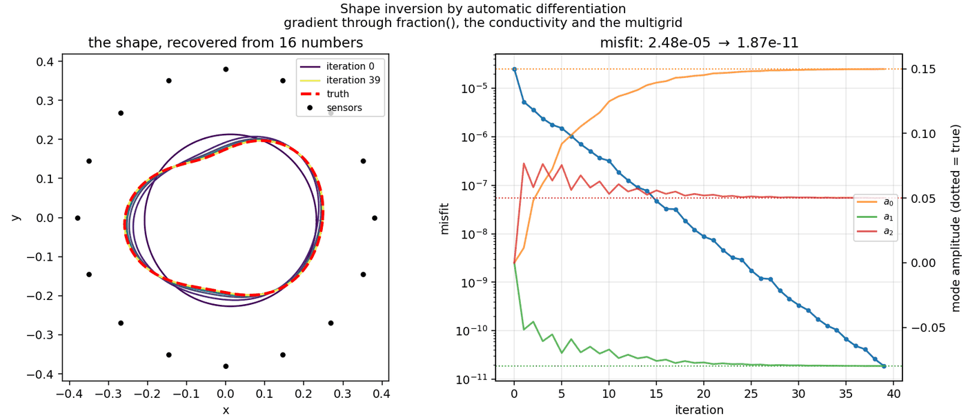
Shape inversion by automatic differentiation.
An inverse problem: recover the shape of an inclusion from sensor measurements around
it. The gradient is obtained by differentiating straight through the whole solver,
including the geometric volume-fraction computation and the multigrid solve, so the
16 shape parameters can be driven by a standard descent. Over 39 iterations the misfit
falls from 2.5 × 10⁻⁵ to
1.9 × 10⁻¹¹, and the recovered mode amplitudes settle
onto their true values.